Tennis Point Leverage

The question

Tennis commentators talk about “big points” as if importance is self-evident. Some of it is: losing at 30–40 is obviously worse than losing at 0–0. What interested me was a harder question—how much does each point move the probability of holding serve, and where do real players depart from a purely mechanical model of the game?

I approached that as a comparison between two systems. The first is an exact probabilistic baseline where every point is an independent Bernoulli trial. The second is a recurrent model trained on real point sequences. The baseline tells me what should happen from the score alone; the LSTM captures what actually tends to happen in the data. The gap between them is where pressure, sequencing, and selection effects begin to show up.

170K

service games

43 pp

leverage at 30–30

+25.6 pp

first-point hold gap

+2.4 pp

observed momentum

Starting at the baseline (pun intended)

Let $H(s,r)$ be the probability that the server holds from score state $(s,r)$, and let $p$ be the server’s probability of winning an individual point. Using the tour-level approximation $p \approx 0.65$, the game can be written as a recurrence:

Deuce is the only cyclic state. If I abbreviate $H_D=H(3,3)$, the recurrence passes through advantage-server and advantage-receiver:

Substituting those advantage states back into deuce produces a fixed-point equation:

Solving for $H_D$ gives the familiar two-points-in-a-row result:

This baseline deliberately assumes away momentum, pressure, player identity, surface, and match context. That is its value: it gives me a clean counterfactual. Any residual has to come from something the independence model does not represent.

Learning the empirical game

I extracted roughly 170,000 non-tiebreak service games from Jeff Sackmann’s Match Charting Project. Each point becomes a three-value observation:

The score features locate the point within the game; the binary outcome lets the model update its belief sequentially. Games are padded to 24 points, and a mask prevents padded timesteps from contributing to the loss.

At each timestep, the LSTM combines the current point with its previous hidden state. The forget, input, and output gates decide what to retain, what to write, and what to expose:

Those gates update the cell state, then the hidden state becomes the input to a small prediction head:

I chose an LSTM over a feed-forward score lookup because two games can reach the same score through different sequences. A basic recurrent network would preserve order too, but it introduces a familiar training problem. For a vanilla RNN,

the gradient reaching an early hidden state contains a product of one Jacobian per later timestep:

If the effective norm of those factors is below one, the gradient decays roughly exponentially with sequence length; above one, it can explode:

The LSTM’s additive cell-state update creates a more direct gradient path. Its local derivative depends on the learned forget gate rather than another multiplication by a fixed recurrent matrix:

When history remains useful, the network can keep $f_t$ near one. That is the practical reason it can carry information through a long deuce sequence more reliably than a basic RNN.

Backpropagation through time still has to combine two sources at every step: the loss emitted at that point and the influence of the hidden state on every future point:

Written at the gate level, the cell gradient accumulates both the current output path and the future cell-state path:

Parameter gradients then sum the contribution from every point in the unrolled game. For the forget gate, for example:

I did not implement those derivatives by hand in the project. PyTorch’s nn.LSTM returns the full $B\times T\times 32$ hidden-state tensor, the prediction head maps every state to a probability, and the masked loss reduces those outputs to one scalar. Calling loss.backward() then traverses the entire unrolled graph. Because a service game is capped at only 24 points, I use full BPTT rather than truncating the sequence.

I trained with binary cross-entropy at every valid timestep—not only at the end of the game—so the network had to produce a useful hold probability throughout the sequence:

Here $m_{i,t}$ is one only for real points, so padding contributes neither loss nor gradient. The final hold/break label $y_i$ is expanded across every valid point in game $i$. Each batch then follows four steps:

1. Pad variable-length games to 24 points and construct the timestep mask.
2. Run the sequence through the LSTM and emit one probability after every point.
3. Apply masked binary cross-entropy against the eventual hold/break outcome.
4. Backpropagate through all valid timesteps and update the weights with Adam.

• 2 LSTM layers with a 32-dimensional hidden state
• 32 → 16 → 1 prediction head with ReLU and sigmoid
• 135,876 training games and 33,970 validation games
• Adam optimizer, learning rate 0.001, batch size 64, 20 epochs

The repository reports 99.2% final-timestep validation accuracy. I treat that as a sanity check rather than the main result: by the final point, the score almost gives away the outcome. The useful object is the full probability path before the game is decided.

Defining leverage

Once the model estimates empirical hold probability $\hat{H}(s,r)$, leverage is the difference between the next state after winning and the next state after losing:

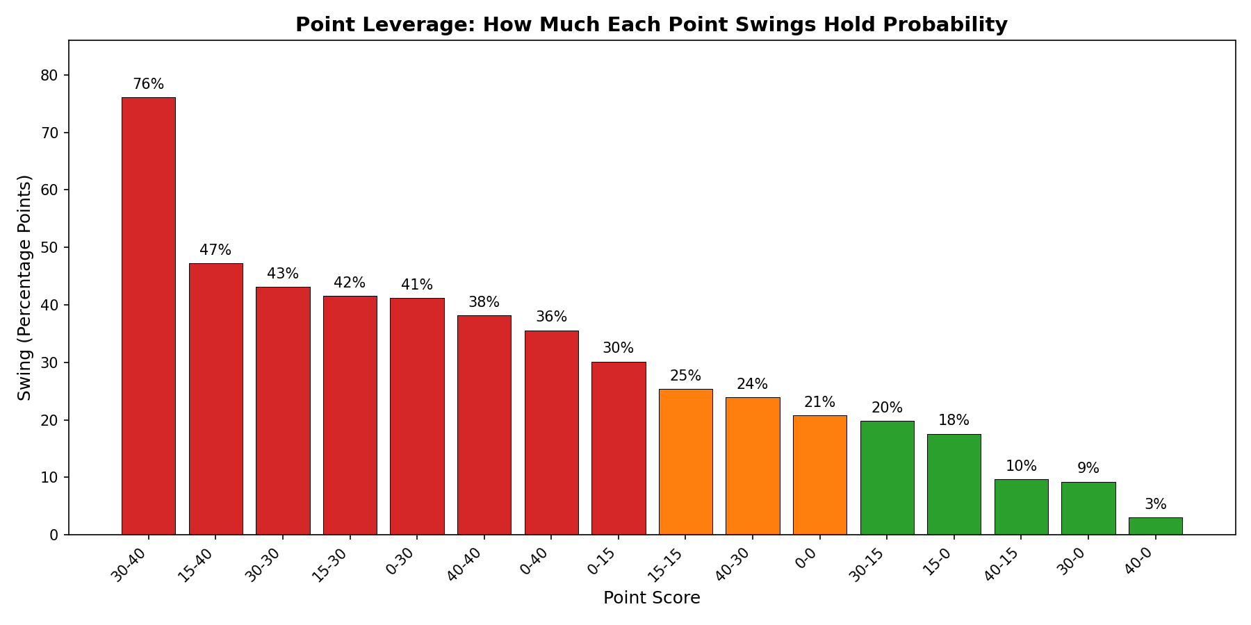
It is a counterfactual swing measured in percentage points. At 30–30, winning moves the server toward game point while losing creates break point. The model estimates a 43-point gap between those branches, making 30–30 the highest-leverage non-terminal state. Earlier pressure states are close: 15–30 produces a 42-point swing and 0–30 a 41-point swing.

Reality minus expectation

To separate score mechanics from observed behavior, I defined performance deviation as the LSTM estimate minus the independent-point baseline:

Positive values mean servers hold more often than the baseline expects; negative values mean they hold less often. The result is not a simple “players are clutch” story. At 15–40, servers outperform by 2.8 percentage points, while at 30–40 they underperform by 3.1 points. At 0–0 the residual is −4.8 points, the largest absolute departure in the standard score grid.

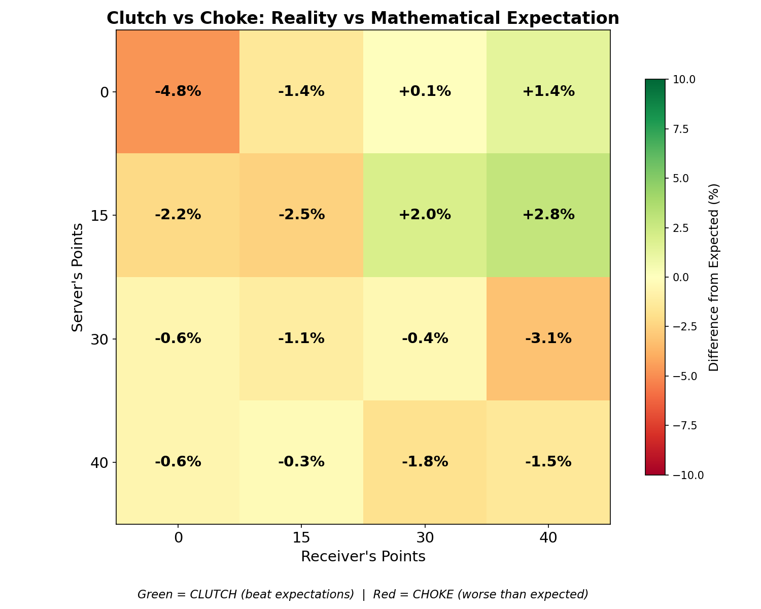
I like this result because it resists the clean headline. Pressure is not a single scalar that switches on at break point. Different score states carry different tactical incentives, samples, and player populations. The residual map is evidence of structure beyond the baseline—not proof of a psychological mechanism.

Two secondary effects

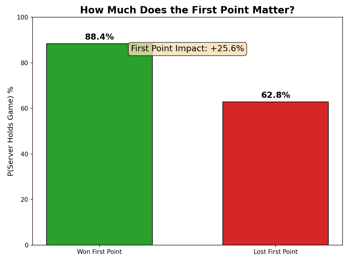
The first point produced the largest simple conditional gap in the analysis:

I also tested short-range momentum by conditioning the current point on the previous point’s outcome across 696,622 transitions:

With that sample size, the difference is statistically detectable, but it is still small in practical terms. More importantly, this conditional comparison is not causal: player quality, serve rotation, and score context can all create persistence without a psychological “hot hand.”

Extending from games to matches

The service-game model answers a deliberately local question. I also wanted to see what “importance” looked like across an entire match, where the same point score means something different depending on the set score, server, tiebreak state, and match format. For that, I built a separate causal Transformer.

Each point is encoded with nine normalized features:

A learned linear projection maps that vector into $d_{\mathrm{model}}=64$ dimensions, then adds sinusoidal positional encoding:

The encoder uses three layers, four attention heads, a 256-dimensional feed-forward sublayer, and 0.1 dropout. Within each head, scaled dot-product attention is:

The mask $M$ is zero on and below the diagonal and $-\infty$ above it. That makes the model causal: the prediction after point $t$ can attend to points $\leq t$, but never to the future. A padding mask separately removes unused positions from shorter matches.

Training follows the same timestep-supervision idea as the LSTM, but at match scale. I split matches chronologically into 80% training, 10% validation, and 10% test sets, padded sequences to 500 points, and optimized masked binary cross-entropy at every timestep. The run used:

• AdamW with learning rate 0.001 and weight decay 0.01
• Cosine learning-rate annealing over 30 epochs
• Batch size 32 and gradient clipping at norm 1.0
• A sigmoid prediction head producing match-win probability after every point

In the saved training history, validation accuracy peaks at 96.2% around epoch 14. After that, training loss continues to fall while validation loss rises—a visible sign of overfitting. The loop saves a checkpoint only when validation accuracy improves, so the analysis can use the best generalizing state rather than assuming the final epoch is the best one.

Once I have the probability path $\hat{p}_1,\ldots,\hat{p}_T$, I define the observed importance of point $t$ as the size of the update it caused:

I call the final crossing of the 50% line the match’s “decision point.” Formally, it is the largest timestep where the predicted favorite changes:

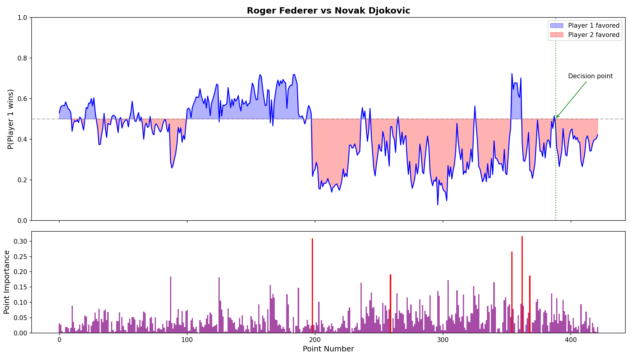
This match is exactly why I wanted the sequence model. Federer spends long stretches above 50%, and several late points produce enormous local probability changes, but the favorite keeps flipping. The green line does not claim that one point caused the outcome; it identifies the last moment when the model’s balance of evidence crossed from one player to the other and never returned.

What I would improve next

The current model pools eras, surfaces, rounds, and players. Charted matches also skew toward prominent players and high-profile events. A stronger follow-up would use hierarchical player effects, surface-specific serve priors, chronological out-of-sample evaluation, and calibration metrics at intermediate score states.

I would also separate prediction from explanation more aggressively. The LSTM is useful because sequence order matters, but the independence baseline remains the most interpretable part of the analysis. The project became interesting when I stopped asking the network for a verdict and started using it as one side of a controlled comparison.